Bartik Instrument

Gains exist, distribution is messy

Aggregate gains from trade are robust across HO, Ricardian, and new-trade models.
Who gains and loses depends on factor mobility.
HO: gains accrue to the abundant factor (Stolper-Samuelson), assuming factors move freely across industries.
SFM (Specific Factor Model): in the short run, some factors are tied to a sector → clear winners and losers.

The textbook distinction in one line

HO: long run, perfect mobility, factor-price equalization.
SFM: short run, sector-specific factors, sectoral wage gaps.
Empirical reality: the “short run” can last a decade or more, and the location of immobile factors is regional.
This is what shift-share designs let us see in the data.

The within-country problem

Cross-country evidence on gains from trade is settled.
Within-country evidence is mixed and politically explosive.
Why? Adjustment is spatial: districts, commuting zones, and provinces specialize in different sectors and absorb shocks differently.
Reasons for imperfect mobility:
- skill mismatch (sector-specific human capital)
- geographic immobility (housing, family ties, language)
- institutional frictions (labor laws, licensing)

What we want to estimate

We want a local causal effect of a trade shock:

$Y_\ell = \alpha + \delta\,X_\ell + \varepsilon_\ell$

$Y_\ell$ — outcome in region $\ell$ (employment, wages, poverty)
$X_\ell$ — local exposure to the trade shock (e.g., change in import penetration)
$\delta$ — the parameter we care about

Problem. $X_\ell$ is endogenous: regions that import more are also regions where productivity, demand, or politics differ in unobserved ways.

→ We need an instrument for $X_\ell$ .

The Bartik (shift-share) idea

Two ingredients:

Shares $s_{\ell k}$ — region $\ell$ ’s pre-period exposure to sector $k$ (employment, output, or expenditure share)
Shifts $g_{k}$ — a common (national or world) shock to sector $k$

Combine into a single regional exposure measure:

$Z_\ell \;=\;\sum_k s_{\ell k}\,g_{k}$

The instrument predicts how hard region $\ell$ should be hit by a common shock, given its industrial structure.

Why call it “Bartik”?

Tim Bartik (1991) used national industry growth rates interacted with local industry mix to predict local labor demand growth.
The construct predates him (Perloff 1957, Freeman 1980) but the name stuck after Blanchard & Katz (1992) popularized it.
In trade: replace national growth with tariff changes (Topalova) or import surges (ADH).
Goldsmith-Pinkham, Sorkin, and Swift (2020) formalize it as a GMM problem with the shares as instruments.

A first numerical look

3 regions × 2 sectors. Tariffs fall between 1987 and 1988.

region	$L_{\text{Agri}}$	$L_{\text{Manuf}}$	$s_{\text{Agri}}$	$s_{\text{Manuf}}$
A	100	9 000	0.011	0.989
B	1 000	400	0.714	0.286
C	700	3 000	0.189	0.811

National tariff change 1987→1988: Agri 30 → 10, Manuf 20 → 5.

Bartik exposure $Z_\ell = s_{\ell,\text{Agri}}\Delta\log t_{\text{Agri}} + s_{\ell,\text{Manuf}}\Delta\log t_{\text{Manuf}}$ :

region	$Z_\ell$ (Δlog)	$Z_\ell$ (Δlevel)
A	−1.38	−15.1
B	−1.18	−18.6
C	−1.33	−15.9

Note the ranking flips: log change makes A most exposed; level change makes B most exposed.

What just happened?

Manuf had the larger proportional cut: $\log(5/20)=-1.39$ vs. $\log(10/30)=-1.10$ .
Agri had the larger absolute cut: $-20$ pp vs. $-15$ pp.
Which one matters? Depends on the outcome model: log-log specifications need $\Delta\log t$ , level specifications need $\Delta t$ .
Lesson: the Bartik is only as well-motivated as the production-side or trade-elasticity model behind it.

First stage, reduced form, IV

The Bartik is used as an instrument:

First stage $\quad X_\ell = \pi_0 + \pi_1 Z_\ell + u_\ell$

Reduced form $\quad Y_\ell = \rho_0 + \rho_1 Z_\ell + v_\ell$

2SLS $\quad \widehat\delta_{\text{IV}} = \rho_1/\pi_1$

Many papers (ADH 2013, Topalova) report the reduced-form coefficient $\rho_1$ directly, calling $Z_\ell$ “exposure.”
The 2SLS scaling requires $\pi_1\neq 0$ and the exclusion restriction $E[Z_\ell \varepsilon_\ell]=0$ .

Identification: two camps

Goldsmith-Pinkham, Sorkin, and Swift (2020) ask the central question: which assumption makes the Bartik valid?

Camp	Source of identification	Champion paper
Share-based	Shares $s_{\ell k}$ are exogenous to unobservables	Goldsmith-Pinkham, Sorkin & Swift (2020)
Shock-based	Shifts $g_k$ are quasi-randomly assigned	Borusyak, Hull & Jaravel (2022)

Both deliver consistent IV under different conditions. The right diagnostic depends on which assumption you lean on.

Share exogeneity (GP framework)

Goldsmith-Pinkham, Sorkin, and Swift (2020) prove: the Bartik 2SLS estimator equals a GMM estimator where each share $s_{\ell k}$ acts as a separate instrument, weighted by Rotemberg weights $\alpha_k$ .

$\widehat\delta_{\text{Bartik}} = \sum_k \alpha_k\,\widehat\delta_k$

$\widehat\delta_k$ — just-identified IV using share $s_{\cdot k}$ alone
$\alpha_k$ — Rotemberg weight, $\sum_k \alpha_k = 1$ , can be negative
A few industries usually carry most of the weight → the design hinges on the exogeneity of those few shares.

Rotemberg weights

For each industry $k$ , the weight is

$\alpha_k \;=\; \frac{g_k \cdot \sum_\ell s_{\ell k}\,X_\ell}{\sum_{k'} g_{k'} \cdot \sum_\ell s_{\ell k'}\,X_\ell}, \qquad \sum_k \alpha_k = 1.$

Two ingredients drive $\alpha_k$ :

size of the shift $g_k$ — industries with bigger national shocks matter more.
first-stage covariance $\sum_\ell s_{\ell k}\,X_\ell$ — how strongly industry $k$ ’s shares correlate with the endogenous regressor.

Weights can be negative: if $g_k$ and the first-stage covariance have opposite signs, that industry pulls the Bartik in the opposite direction. A handful of industries usually carry most of the weight.

Named for Julio Rotemberg (1983), who used the same decomposition logic in a different IV setting; Goldsmith-Pinkham, Sorkin, and Swift (2020) formalised it for the Bartik.

Rotemberg weights: 2x2

Use our toy data. Set $X_\ell = Z_\ell^{\text{lev}}$ so the mechanics are visible: $X_A=-15.1,\,X_B=-18.6,\,X_C=-15.9$ , with shifts $g_{\text{Agri}}=-20,\,g_{\text{Manuf}}=-15$ .

First-stage covariances:

$\textstyle\sum_\ell s_{\ell,\text{Agri}} X_\ell = 0.011(-15.1)+0.714(-18.6)+0.189(-15.9) = -16.45$ $\textstyle\sum_\ell s_{\ell,\text{Manuf}} X_\ell = 0.989(-15.1)+0.286(-18.6)+0.811(-15.9) = -33.15$

Numerators: $(-20)(-16.45)=329.0$ and $(-15)(-33.15)=497.2$ . Denominator $826.2$ .

$\boxed{\alpha_{\text{Agri}}=0.40,\qquad \alpha_{\text{Manuf}}=0.60.}$

Manufacturing carries 60% of the Bartik. With 100+ industries in Topalova or ADH, 5–10 industries typically carry 80% of the weight — those are the shares whose exogeneity you actually need to defend.

Rotemberg weights in R

# shares: L × K matrix; g: length K; X: length L
fs_cov <- as.numeric(t(shares) %*% X)          # first-stage covariances
alpha  <- g * fs_cov
alpha  <- alpha / sum(alpha)                   # Rotemberg weights

# per-industry just-identified IV
beta_k <- as.numeric(t(shares) %*% Y) / fs_cov
sum(alpha * beta_k)                            # = Bartik 2SLS estimate

The bartik.weight package (GitHub: paulgp/bartik-weight) does this and produces the Goldsmith-Pinkham, Sorkin, and Swift (2020) Table 5 diagnostic panel directly.

Diagnostics from Rotemberg weights

Goldsmith-Pinkham, Sorkin, and Swift (2020) recommend reporting:

Concentration of weights — Herfindahl of $|\alpha_k|$ . If 2–3 industries dominate, your identification is really about those industries.
Top-5 industries — list them and ask: are their shares plausibly exogenous to local outcome trends?
Pre-trend checks on $Z_\ell$ — does pre-shock $Z_\ell$ predict pre-shock changes in $Y_\ell$ ?
Just-identified IV by industry — if $\widehat\delta_k$ varies wildly across top industries, the pooled estimate is fragile.

Shock exogeneity (BHJ framework)

Borusyak, Hull, and Jaravel (2022) take a different route. Treat the shifts $g_k$ as random and the shares as exposure weights.

Identification: $g_k$ is uncorrelated with sector-average residuals.
Works well when shifts come from outside the system you study (e.g., supply-driven Chinese import surge from China’s TFP and WTO accession).
Diagnostic: tests for shock balance — does $g_k$ correlate with pre-shock industry characteristics?
The ADH “instrument with other rich countries’ imports from China” exploits exactly this — it isolates the supply-driven component of the shock.

Inference: don’t use OLS standard errors

Adão, Kolesár, and Morales (2019) show that conventional cluster-robust SEs over-reject with shift-share regressors:

Residuals are correlated across regions that share industry mix.
Their fix: an exposure-robust SE that treats industries as the clusters of randomness.
In R, you can implement AKM SEs via the ShiftShareSE package or replicate by IV with industry-level data.
Rule of thumb for class: if you see Bartik with white SEs only, be skeptical.

Limitations to keep in mind

Pre-period shares can be endogenous (industries locate for a reason).
Common shocks may be heterogeneous across sub-periods → time-varying $g_k$ .
Placebo tests on pre-period $Y$ are essential.
Weighting: by region size, by inverse SE, by employment — affects which observations drive the result.
Aggregation matters: districts vs. provinces vs. commuting zones give different answers.

Topalova (2010): India 1991

India’s 1991 liberalization cut tariffs unevenly across industries.
Cross-district variation in pre-reform industry mix → cross-district variation in exposure.
Difference-in-differences with Bartik exposure as the treatment.

Identification: the pace of tariff cuts was dictated by external (IMF) pressure and was negotiated industry-by-industry without regard to district outcomes → shocks plausibly exogenous to district trends.

Topalova: instrument

$Z_\ell^{\text{Top}} = \sum_k s_{\ell k}^{\,1987}\,\Delta\log(\text{Tariff}_k)$

$s_{\ell k}^{1987}$ — district $\ell$ ’s pre-reform employment share in industry $k$
$\Delta\log(\text{Tariff}_k)$ — national log-change in industry $k$ ’s tariff between 1987 and 1997

Outcomes: district-level poverty headcount, poverty gap, consumption growth.

Topalova: specification

Topalova runs a panel across four NSS rounds (1983, 1987–88, 1993–94, 1999–2000):

$Y_{dt} = \alpha_d + \gamma_{st} + \delta\,\text{Tariff}_{dt} + \mathbf{W}'_{dt}\lambda + \varepsilon_{dt}$

with district tariff constructed Bartik-style,

$\text{Tariff}_{dt} = \sum_k s_{dk,1987}\cdot \text{Tariff}_{kt}$

$\alpha_d$ — district FE (kill all time-invariant district traits)
$\gamma_{st}$ — state × year FE (absorb state-wide trends)
shares frozen at 1987; national tariffs $\text{Tariff}_{kt}$ vary year-by-year
IV: instrument realised tariffs with the scheduled tariff reduction path

Under two-way FE this is numerically equivalent to a long-difference regression on $\Delta Y_d$ vs. $\Delta\text{Tariff}_d$ — which is why ADH-style papers (and teaching slides) often present Bartik in differences.

Topalova: findings

Rural districts more exposed to tariff cuts → slower decline in poverty, lower consumption growth.
Effect concentrated among the geographically immobile and least skilled.
Mechanism: rigid labor laws → costly to fire and to expand → factor reallocation stalls.
In states with flexible labor regulation, the poverty effect of exposure is statistically zero.

Takeaway: Bartik captures exposure; institutions decide adjustment.

Autor, Dorn & Hanson (2013): the China shock

Autor, Dorn, and Hanson (2013) examine US commuting zones (CZs) 1990–2007.
China’s WTO accession (2001) and supply-side reforms drove a sustained import surge.
Variation across CZs comes from pre-shock industry mix.

ADH: the instrument

$\Delta IPW_{c\tau} = \sum_k \frac{L_{ck,t_0}}{L_{k,t_0}}\cdot \frac{\Delta M^{US}_{k\tau}}{L_{c,t_0}}$

$L_{ck,t_0}$ — start-of-period employment in CZ $c$ , industry $k$
$\Delta M^{US}_{k\tau}$ — change in US imports from China in industry $k$

To address shock endogeneity (US demand could pull in imports too), ADH instrument $\Delta M^{US}$ with $\Delta M^{OTH}$ — imports from China to eight other rich countries. This isolates the China-side supply shock.

ADH: main results

High-exposure CZs lose more manufacturing jobs.
Wages fall, esp. among non-college workers.
No offsetting employment gains in other sectors at the local level.
Effects persist for at least a decade.
Autor, Dorn, and Hanson (2016) (2016 review) extends to job churning, lifetime earnings, social spending, marriage rates, mortality.

Why ADH matters methodologically

Cleanest example of the shock-based identification logic in BHJ.
The “other rich countries” instrument is the canonical move for purging demand-side endogeneity from a Bartik.
Sparked the AKM (2019) literature on inference because their headline SEs were too tight.
Their data and Stata replication files are widely used in teaching.

Kis-Katos & Sparrow (2015): Indonesia 1993–2002

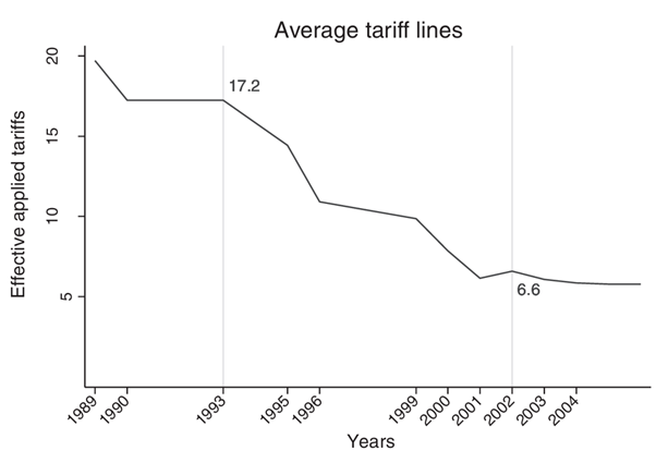
259 districts; outcome is district-level poverty.
Two waves of tariff cuts: WTO 1995 + IMF program 1999.
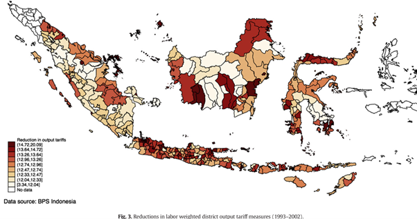
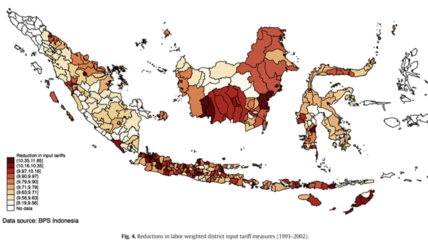
Innovation: separate output and input tariff exposure using a 1990 input-output table.

Output vs. input tariffs

$Ot_{kt}=\sum_{s=1}^S \left(\frac{Q_{sk,t=0}}{Q_{k,t=0}}\times t_{st}\right)$

$It_{kt}=\sum_{s=1}^S \left(\frac{Q_{sk,t=0}}{Q_{k,t=0}}\times \sum_{j=1}^J \frac{M_{js,1990}}{M_{s,1990}} t_{jt} \right)$

sector $s$ , district $k$ , time $t$ , input sector $j$ , labor $Q$ , tariff $t$

The first share weights output tariffs by district industry mix; the second additionally weights through the I-O matrix to capture imported intermediate inputs embodied in each sector.

Output tariff exposure

Input tariff exposure

Kis-Katos & Sparrow: findings

$\Delta y_{kt}=\alpha + \beta_1 Ot_{kt} + \beta_2 It_{kt} + \gamma \Delta X'_{kt} + I'_k \theta + \lambda_{rt} + \Delta \epsilon_{kt}$

$\beta_1 > 0$ — output tariff cuts raise poverty (import competition story).
$\beta_2 < 0$ and larger in magnitude — input tariff cuts reduce poverty (cheaper intermediates → firm competitiveness → low-skill work participation and middle-skill wages rise).

Net effect on Indonesian poverty is negative — but only because input tariff liberalization dominates. The distributional story matters.

Three applications side by side

	Topalova (2010)	ADH (2013)	KK & Sparrow (2015)
Country	India	US	Indonesia
Episode	1991 reform	1990–2007	1993–2002
Unit	districts	commuting zones	districts (259)
Shock	tariff cuts	China imports	tariff cuts (2 waves)
Share	1987 employment	start-period emp.	I-O × employment
Outcome	poverty, consumption	jobs, wages	poverty
Direction	exposure ↑ → poverty ↑	exposure ↑ → jobs ↓	output↑ poverty↑, input↓ poverty↓