Tariff and Non-Tariff Measures: Heterogenous Impacts on Productivity of Indonesian firms
Krisna Gupta
Crawford PhD Seminar
October 2, 2020
Arianto Patunru, Paul Gretton, Budy Resosudarmo
Content
- introduction
- literature review
- data
- method
- results
- discussion & policy recommendations
Introduction
Introduction
Indonesia relies in manufacturing sector to boost growth
Emphasize on tech upgrade
also on export-led growth
This means more openness:
- financing R&D
- import ⇒⇒ tech-upgrade (Castellani and Fassio 2019)
Source: kemenperin.go.id
Trend is on the opposite
However, Protectionism is on the rise, including in Indonesia (Patunru 2018)
Since GFC, While overall tariff went down, Non-Tariff Measures went up
The role of Ministry of Industry is increasing (e.g., National Standards (SNI) and Local Content Requirement (LCR)) (Munadi 2019)
Pandemic has accelerated the trend, potentially using tariff as well
Protectionism policies may lead to more policies:
- US trade war Case: iron ⇒⇒ appliances
- Indonesian Case: corn & soybean ⇒⇒ chicken, mobile phone
Introduction
- The straightforward question:
To what extent tariff and NTMs affect firm's productivity?
Further investigation is conducted:
does size matter? (core question since Melitz (2003))
how does protectionism affect employment?
can NTMs reduces firms' imports in general?
Building from Amiti and Konnings (2007), I estimate TFP and use it as the dependent variable
Key data sources:
- Tariff data are scrapped from MoF regulations
- NTM from TRAINS database
- Firm's characteristics & trade: Survei Industri and Customs data from BPS from 2008 to 2012
Brief Literature Review
On trade and industry
On the role of international trade and trade policies to firm's performance, literature is abundant:
- Help firm access better inputs (Amiti and Konings 2007; Bas and Strauss-Kahn 2014; Castellani and Fassio 2019; Ing, Yu and Zhang 2019)
- Help firms innovate and be more productive (Bas and Strauss-Kahn 2014, Pierola, Fernandez and Farole 2018; Ing, Yu and Zhang 2019; Pane and Patunru 2019)
- Help firms from developing countries access the more lucrative foreign markets (An and Maskus 2009; Cadot et al. 2015; Fugazza, Olarreaga and Ugarte 2017)
How to measure performance of industries and firms:
- most of the literature uses export (value, quantity, price, scope)
- some criticism includes endogeneity and the role of export to more meaningful metrics (such as GDP, employment and wage)
- The alternative is using TFP (Amiti and Konings 2007; Pane and Patunru 2019)
On Using TFP
Using TFP is preferable (Indonesian context):
Trade policy is arguably 'less endogenous' to firm's TFP:
- Indonesian government often aim for CAD (Patunru 2018), not firms TFP.
- Manufacturing Firms' influence over tariff is less strong (Amiti and Konings 2007; Mobarak and Purbasari 2005)
Firm's TFP is a more meaningful metric than export
TFP estimation:
- non-linear method (Henningsen and Henningsen 2012) has less restriction, but it is harder to converge and contain less economic intuition.
- Linear method is preferable but endogeneity needs to be treated:
- using investment proxy (Olley and Pakes 1998)
- using intermediate input proxy (Amiti and Konings 2007; Levinsohn and Petrin 2003)
On Trade Policies
- The impact of tariff is established, but NTM's impact is mixed (Kee et al. 2009; Cadot et al. 2015)
On NTMs:
Price-difference method & Indonesian context (Marks 2018):
- NTMs correlate with higher domestic price
- Hard to get consistent data on price
- possibility that price reflects quality
Most are using categorical variable with AVE-style estimation
UNCTAD (2017) built an NTM database called TRAINS:
- Less judgmental (NTM vs NTB)
- lack depth (Cadot et al. 2015)
Data
Firms
Survei Industri (SI), BPS
- follows many Indonesian manufacturing since 1970s
- infos include factor used, foreign ownership, output, fraction of export and import
- unbalanced, unfortunately
- Inconsistent fixed asset and energy consumption
Customs data
- 2008-2012 with firm id to integrate with SI
- varies with countries and HS-8-digit
- not exactly match one-on-one with SI
- can't say for sure if the import is directly used for production
Not all firms reporting export and import in SI exist in the customs data, and vice-versa
- may be using third party traders
Firms' Characteristics
Table 1. Firms' characteristics, 2008-2012
| Characteristics | All_SI | Non_customs | Customs_only |
|---|---|---|---|
| foreign ownership (%) | 8.15 | 5.96 | 34.77 |
| (26.17) | (22.60) | (45.06) | |
| fraction of output exported (%) | 0.23 | 0.21 | 0.4 |
| fraction of output exported | (37.52) | (0.37) | (0.42) |
| fraction of input imported (%) | 0.08 | 0.07 | 0.31 |
| (0.24) | (0.21) | (0.38) | |
| no. of labour employed | 191.07 | 162.75 | 535.44 |
| (711.73) | (602.46) | (1,457.65) | |
| capital stock (Million IDR) | 198 | 194 | 250 |
| (44,800.00) | (46,500) | (10,400) | |
| total intermediate input (Million IDR) | 50.8 | 41 | 170 |
| (617.00) | (515) | (1,330) | |
| total output (Million IDR) | 90.3 | 73.3 | 296 |
| (958.00) | (861) | (1,740) | |
| total value added (Million IDR) | 38.5 | 31.6 | 123 |
| (455.00) | (414) | (789) | |
| value added per labour (IDR) | 137,987.10 | 126,074 | 282,857 |
| (2,515,300.00) | (2,600,177) | (1,012,159) | |
| No. of observation | 117,598 | 108,662 | 8,915 |
Average number of SPS is the highest
Table 2. Mean (St.Dev) of each NTM for all HS-6-digits
| NTM | Codes | N2008 | N2009 | N2010 | N2011 | N2012 | Examples |
|---|---|---|---|---|---|---|---|
| Sanitary & Phytosanitary (SPS) | A | 1.715 | 2.337 | 2.222 | 2.255 | 2.774 | Authorization requirements |
| (2.644) | (4.018) | (3.950) | (4.054) | (5.128) | Quarantine requirements | ||
| Technical Barrier to Trade (TBT) | B | 0.481 | 0.455 | 0.641 | 0.682 | 0.663 | Testing requirements |
| (0.962) | (0.978) | (1.334) | (1.361) | (1.352) | labeling requirements | ||
| Pre-shipment inspections and other formalities | C | 0.562 | 0.466 | 0.443 | 0.462 | 0.776 | pre-shipment inspection |
| (1.202) | (1.081) | (1.059) | (1.046) | (1.075) | only trough specific ports | ||
| Non-automatic licensing, quotas, QC, etc | E | 0.623 | 0.56 | 0.605 | 0.618 | 0.594 | licensing |
| (0.809) | (0.818) | (0.873) | (0.861) | (0.853) | quota | ||
| Price-control measures, extra taxes, charges | F | 0 | 0 | 0.015 | 0.014 | 0.016 | customs service fee |
| (0.000) | (0.000) | (0.168) | (0.165) | (0.168) | consumption tax | ||
| Measures affecting competition | H | 0.019 | 0.052 | 0.05 | 0.048 | 0.046 | Only SOEs |
| (0.139) | (0.238) | (0.233) | (0.229) | (0.224) | - | ||
| Export-related measures | P | 0.901 | 0.704 | 0.708 | 0.683 | 1.172 | export permit |
| (1.172) | (1.132) | (1.109) | (1.098) | (1.465) | export quota | ||
| observations | - | 1,675 | 2,204 | 2,318 | 2,400 | 2,510 | - |
Simple average of tariffs from 2008-2012
Table 3. Tariff from MoF regulations (left) compared to WITS (right)
| Kind | T2008 | T2009 | T2010 | T2011 | T2012 |
|---|---|---|---|---|---|
| MFN | 7.049 | 7.612 | 6.928 | 6.975 | 6.96 |
| (12.213) | (12.536) | (8.037) | (7.231) | (7.145) | |
| ASEAN | 2.478 | 2.49 | 0.15 | 0.15 | 0.15 |
| (11.094) | (11.206) | (4.559) | (4.559) | (4.559) | |
| China | 7.049 | 3.819 | 2.193 | 2.208 | 1.941 |
| (12.213) | (12.673) | (7.941) | (7.941) | (7.927) | |
| South Korea | 7.049 | 2.624 | 1.912 | 1.912 | 1.542 |
| (12.213) | (12.265) | (7.131) | (7.131) | (7.102) | |
| India | 7.049 | 7.612 | 6.394 | 5.874 | 5.341 |
| (12.213) | (12.536) | (7.809) | (7.517) | (7.322) | |
| Japan | 6.11 | 4.639 | 3.274 | 2.618 | 2.23 |
| (11.967) | (12.356) | (7.353) | (7.114) | (6.487) | |
| ANZ | 7.049 | 6.446 | 2.948 | 2.278 | 1.545 |
| (12.213) | (11.922) | (6.765) | (6.318) | (6.065) |
| Kind | T2008 | T2009 | T2010 | T2011 | T2012 |
|---|---|---|---|---|---|
| MFN | 7.762 | 7.595 | 7.564 | 7.051 | 7.053 |
| (12.631) | (12.456) | (12.412) | (7.015) | (7.016) | |
| ASEAN | - | 1.84 | 1.843 | 0.152 | 0.152 |
| (11.079) | (11.067) | (4.285) | (4.287) | ||
| China | 3.665 | 2.743 | 1.85 | 1.579 | |
| (12.342) | (12.392) | (6.853) | (6.823) | ||
| South Korea | 2.564 | 2.56 | 1.698 | 1.326 | |
| (12.087) | (12.084) | (6.395) | (6.349) | ||
| India | - | - | 5.409 | 4.991 | |
| (6.726) | (6.620) | ||||
| Japan | - | - | |||
| ANZ | |||||
Method
TFP estimation
The framework uses two-stage regression:
first, estimating TFP
yit=β0+βllit+βkkit+βmmit+βnnit+ϵityit=β0+βllit+βkkit+βmmit+βnnit+ϵit
where:
yityit = log of revenue of firm i at time t
litlit = log of number of labour
kitkit = log of fixed assets
mitmit = log of intermediate materials
nitnit = log of energy consumption
Use the coefficient to predict TFP:
TFPit=yit−ˆβllit−ˆβkkit−ˆβmmit−ˆβnnitTFPit=yit−^βllit−^βkkit−^βmmit−^βnnit then estimate the second stage:
TFPit=γ0+γtarifftariffit+γNTMNTMit+ηitTFPit=γ0+γtarifftariffit+γNTMNTMit+ηit
Some problems
let ϵit=ωit+μitϵit=ωit+μit
where μitμit is iid, while ωitωit is a productivity shock observed only by managers and may correlate with production decisions.
Olley and Pakes (1996) suggest ωitωit follows a first order Markov process and affects a firm's decision on how much to invest (or divest)
Iit=i(kit,ωit)Iit=i(kit,ωit) inversed:
ωit=ϕ(Iit,kit)ωit=ϕ(Iit,kit) Weaknesses of using investment (Levinsohn and Petrin 2003):
- zero investment featured in many datasets (including SI)
- less flexible compared to intermediate input
Lvinsohn-Petrin Method
Levinsohn and Petrin (2003) suggest using intermediate input
ωit=ϕ(mit,kit)ωit=ϕ(mit,kit) Therefore, the first-stage becomes:
yit=β0+βllit+βnnit+ϕ(mit,kit)+μityit=β0+βllit+βnnit+ϕ(mit,kit)+μit Then proceed as follows to estimate TFP.
TFPit=yit−ˆβllit−ˆβkkit−ˆβmmit−ˆβnnitTFPit=yit−^βllit−^βkkit−^βmmit−^βnnit
The command levpet in Stata allows for practical use of the LP method (Petrin, Poi and Levinsohn 2005).
Trade policy variable
The dataset allows for multiple goods imported for each firm. The most practical way is to use coverage ratios.
Tit=∑tariffscVsc∑Vsc∗100Tit=∑tariffscVsc∑Vsc∗100 where:
- Tit=Tit= tariff coverage ratio of firm i at time t,
- tariffsc=tariffsc= tariff imposed on good s from country c at time t
- Vsc= value of good s imported from country c by firm i at time t
And for NTMs:
Cθit=∑NTMθscVsc∑Vsc∗100
where NTMθsc is the number of NTM θ imposed on good s from country c
Coverage ratio
- Table 5 shows simple mean (a) and coverage ratios (b)
- As expected, tariffs lie between MFN and FTAs
- Import licenses and quotas are more important than SPS and TBT
- Coverage ratios vs simple mean:
- no visual difference on tariff
- firms import more goods with NTMs
Table 5a. Simple average
| Variable | Mean | St.Dev. | Min | Max |
|---|---|---|---|---|
| Tariff | 3.503 | 4.971 | 0 | 150 |
| SPS (A) | 0.108 | 0.718 | 0 | 29 |
| TBT (B) | 0.140 | 0.663 | 0 | 13 |
| Pre-shipment inspection (C) | 0.028 | 0.214 | 0 | 5 |
| Licensing, quota, etc (E) | 0.321 | 0.550 | 0 | 6 |
| Price control etc (F) | 0.000 | 0.008 | 0 | 2 |
| Competition measures (H) | 0.007 | 0.083 | 0 | 2 |
| Export-related (P) | 0.063 | 0.376 | 0 | 7 |
Table 5b. Coverage Ratio
| Variable | Mean | St.Dev. | Min | Max |
|---|---|---|---|---|
| Tariff Coverage Ratio (T) | 3.420 | 5.646 | 0 | 150 |
| Coverage ratio A | 0.246 | 0.931 | 0 | 19 |
| Coverage ratio B | 0.202 | 0.478 | 0 | 9 |
| Coverage ratio C | 0.059 | 0.237 | 0 | 4 |
| Coverage ratio E | 0.337 | 0.468 | 0 | 6 |
| Coverage ratio F | 0.000 | 0.001 | 0 | 0 |
| Coverage ratio H | 0.014 | 0.083 | 0 | 1 |
| Coverage ratio P | 0.110 | 0.353 | 0 | 7 |
Second-Stage
The second stage regression then:
tfpit=γ0+γTtit+∑θγθcθit+FOit+αi+ISICi+ηit
Where:
- tfpit=log(TFPit)
- tit=log(1+Tit)
- cθit=log(1+Cθit)
- FOit= foreign ownership of firm i at time t (%)
along with firm's fixed effect and ISIC dummy.
Results
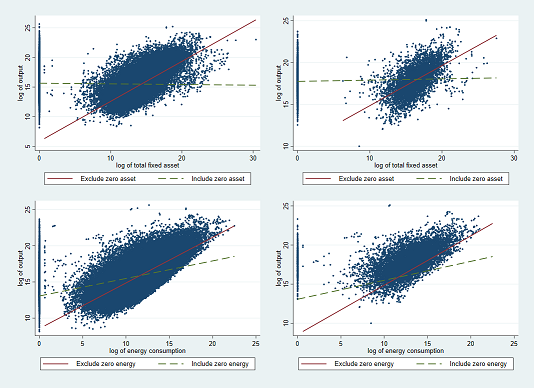
Zero capital problem
Zero capital and energy consumption exists both for SI observations (left) and customs data (right).
TFP Results
- k,n=0 have smaller RTS and much smaller coefficient for k and n
- Lose ± 30% of observations
table 6a. k,n≥0
| Variables | All_SI | Non_customs | Customs_only |
|---|---|---|---|
| Labour (l) | 0.354*** | 0.355*** | 0.268*** |
| (0.005) | (0.005) | (0.011) | |
| Capital (k) | 0 | 0 | 0 |
| (0.000) | (0.000) | (0.002) | |
| Energy (n) | 0.035*** | 0.037*** | 0.019*** |
| (0.001) | (0.001) | (0.003) | |
| input (m) | 0.234*** | 0.251*** | 0.344*** |
| (0.013) | (0.017) | (0.056) | |
| RTS | 0.623 | 0.643 | 0.631 |
| Obs | 117,598 | 108,662 | 8,936 |
Table 6b. k,n>0
| Variables | All_SI | Non_customs | Customs_only |
|---|---|---|---|
| Labour (l) | 0.307*** | 0.307*** | 0.254*** |
| (0.005) | (0.006) | (0.015) | |
| Capital (k) | 0.223*** | 0.219*** | 0.161*** |
| (0.014) | (0.015) | (0.038) | |
| Energy (n) | 0.114*** | 0.114*** | 0.097*** |
| (0.003) | (0.002) | (0.008) | |
| input (m) | 0.281*** | 0.255*** | 0.226*** |
| (0.024) | (0.024) | (0.075) | |
| RTS | 0.925 | 0.895 | 0.738 |
| Obs | 73,265 | 68,294 | 4,971 |
TFP Results
- table 7a over-estimates TFPs
- 3 TFPs are used. 2 from the row customs only, table 7b:
- TFP1 = estimated together with other firms in SI (all_SI)
- TFP2 = estimated within customs only firms (customs_only)
- Value added per labour is used for robustness check
table 7a. TFP with k,n=0
| Variables | All_SI | Non_customs | Customs_only |
|---|---|---|---|
| TFP all SI | 241,611.20 | - | - |
| (4,444,240) | |||
| Non customs | 221,284.30 | 216,246.40 | |
| (4,542,027) | (4,361,599) | ||
| Customs only | 488,787.80 | - | 341,643.80 |
| (3,000,124) | (8,542,388) | ||
| Va/L | 137,987.1 | 126,073.5 | 282,856.5 |
| (2,515,300) | (2,600,177) | (1,012,159) | |
| obs | 117,598 | 108,662 | 8,936 |
Table 7b. TFP with k,n>0
| Variables | All_SI | Non_customs | Customs_only |
|---|---|---|---|
| TFP all SI | 107,036.90 | - | - |
| (2,792,543) | |||
| Non customs | 98,534.27 | 115,020.70 | |
| (2,826,922) | (2,719,907) | ||
| Customs only | 210,429.20 | - | 177,280.20 |
| (2,331,985) | (4,609,524) | ||
| Va/L | 111,455.8 | 100,510.9 | 261,822.6 |
| (2,538,721) | (2,614,048) | (1,043,383) | |
| obs | 73,265 | 68,294 | 4,971 |
Adding size to the regression
Firms in the customs data (possibly) are different
- they are generally bigger, and bigger firms may have ways to offset trade costs
if size matters, it can be discovered using size interaction.
lit=log(Labourit) is used as a proxy
size_tfpit=tfpit+γTtit∗lit+∑θcθit∗lit
- In all:
- 4,971 observations of 1,512 firms
- only customs, k,n>0
- TFP1 estimated with all SI
- TFP2 estimated only customs
- VaL=ValueAddedLabour
results (Right=Left with FE)
| Variables | TFP1 | TFP2 | VaL |
|---|---|---|---|
| tariff | -0.357*** | -0.630*** | 0.071 |
| (0.067) | (0.065) | (0.090) | |
| tariff.l | 0.061*** | 0.112*** | -0.026 |
| (0.012) | (0.011) | (0.017) | |
| SPS | -0.250 | -0.517** | -0.124 |
| (0.234) | (0.260) | (0.381) | |
| SPS.l | 0.026 | 0.076* | -0.008 |
| (0.042) | (0.046) | (0.067) | |
| TBT | 0.213 | 0.194 | 0.486 |
| (0.483) | (0.419) | (0.408) | |
| TBT.l | 0.014 | 0.012 | -0.019 |
| (0.083) | (0.072) | (0.067) | |
| Pre-shipment inspection | 0.418 | 0.749 | -0.005 |
| (0.531) | (0.558) | (0.758) | |
| Pre-shipment inspection.l | -0.058 | -0.116 | 0.051 |
| (0.094) | (0.098) | (0.134) | |
| licensing | -0.650** | -1.444*** | 0.640* |
| (0.266) | (0.263) | (0.371) | |
| licensing.l | 0.107** | 0.258*** | -0.119* |
| (0.047) | (0.046) | (0.064) |
| Variables | TFP1 | TFP2 | VaL |
|---|---|---|---|
| tariff | -0.205** | -0.371*** | 0.259** |
| (0.083) | (0.077) | (0.104) | |
| tariff.l | 0.036** | 0.068*** | -0.048** |
| (0.015) | (0.014) | (0.019) | |
| SPS | -0.260 | -0.381 | 0.103 |
| (0.297) | (0.278) | (0.372) | |
| SPS.l | 0.043 | 0.062 | -0.029 |
| (0.051) | (0.048) | (0.064) | |
| TBT | 0.124 | 0.074 | 0.462 |
| (0.330) | (0.310) | (0.415) | |
| TBT.l | 0.011 | 0.013 | -0.051 |
| (0.058) | (0.055) | (0.073) | |
| Pre-shipment inspection | -0.115 | 0.16 | -0.637 |
| (0.520) | (0.488) | (0.652) | |
| Pre-shipment inspection.l | 0.01 | -0.043 | 0.1 |
| (0.093) | (0.087) | (0.117) | |
| licensing | -0.451 | -0.896*** | 1.477*** |
| (0.311) | (0.292) | (0.390) | |
| licensing.l | 0.065 | 0.147*** | -0.295*** |
| (0.056) | (0.052) | (0.070) |
Results (Right=Left with FE)
| Variables | TFP1 | TFP2 | VaL |
|---|---|---|---|
| price control | -8,559*** | -12,147*** | -29,052*** |
| (3,235) | (2,984) | (4,029) | |
| price control.l | 1,383*** | 1,985*** | 4,718*** |
| (514) | (474) | (640) | |
| competition | -1.155 | -0.693 | -2.269* |
| (1.152) | (1.095) | (1.194) | |
| competition.l | 0.228 | 0.129 | 0.434** |
| (0.216) | (0.210) | (0.213) | |
| export-related | -0.341 | -0.475 | 0.343 |
| (0.357) | (0.385) | (0.679) | |
| export-related.l | 0.066 | 0.095 | -0.049 |
| (0.062) | (0.066) | (0.125) | |
| dummy FDI | 0.157*** | 0.152*** | 0.156** |
| (0.059) | (0.052) | (0.073) | |
| foreign ownership | 0.039*** | 0.040*** | 0.045*** |
| (0.013) | (0.012) | (0.016) | |
| R-sq | - | - | - |
| Variables | TFP1 | TFP2 | VaL |
|---|---|---|---|
| price control | -7,559 | -10,221 | -25,902 |
| (41,100) | (38,558) | (51,565) | |
| price control.l | 1,214 | 1,666 | 4,154 |
| (6,533) | (6,129) | (8,197) | |
| competition | -2.027 | -2.204* | -4.609*** |
| (1.277) | (1.198) | (1.602) | |
| competition.l | 0.393* | 0.413** | 0.834*** |
| (0.220) | (0.206) | (0.276) | |
| export-related | -0.096 | -0.291 | 0.48 |
| (0.476) | (0.446) | (0.597) | |
| export-related.l | 0.036 | 0.075 | -0.073 |
| (0.083) | (0.078) | (0.104) | |
| dummy FDI | 0.066 | 0.061 | -0.022 |
| (0.066) | 0.062 | (0.083) | |
| foreign ownership | 0.023 | 0.024* | 0.025 |
| (0.015) | (0.014) | (0.019) | |
| R-sq | 0.029 | 0.041 | 0.07 |
Employment effect
Results from VaL is confusing
- Perhaps employment is more sensitive to change in production cost compared to reported value added?
Use change in labour as LHS with the consequence of losing 2008
Δlt=log(Lt)−log(Lt−1) Four regressions are conducted, involving:
- No size interaction (L0) and with size interaction (L1)
- with firm, year, ISIC FE and without FE
Employment effect
| Variables | L0 | L0FE | L1 | L1FE |
|---|---|---|---|---|
| tariff | -0.008 | -0.028 | -0.260*** | -1.368*** |
| (0.009) | (0.021) | (0.047) | (0.063) | |
| SPS | -0.028 | -0.120* | -0.176 | -1.650*** |
| (0.020) | (0.066) | (0.153) | (0.230) | |
| TBT | 0.034 | -0.075 | 0.064 | 0.452* |
| (0.038) | (0.075) | (0.236) | (0.257) | |
| Pre-shipment | -0.041 | 0.121 | 0.066 | 1.997*** |
| (0.040) | (0.100) | (0.349) | (0.370) | |
| licensing | -0.015 | -0.042 | -0.818*** | -4.455*** |
| (0.033) | (0.073) | (0.190) | (0.237) | |
| Price-control | 135 | 1,543 | 14,832*** | 6,015 |
| -88 | -1,185 | (4,381) | -25,570 | |
| competition | 0.072 | 0.094 | -0.999 | -2.788*** |
| (0.289) | (0.387) | (1.563) | (1.006) | |
| Export-related | -0.017 | 0.097 | -0.246 | -0.617* |
| (0.028) | (0.091) | (0.203) | (0.333) | |
| foreign dummy | 0.031 | 0.147** | 0.028 | 0.091* |
| (0.030) | (0.065) | (0.031) | (0.053) | |
| observations | 3,726 | 3,726 | 3,726 | 3,726 |
| Variables | L0 | L0FE | L1 | L1FE |
|---|---|---|---|---|
| tariff*l | - | - | 0.043*** | 0.251*** |
| (0.008) | (0.011) | |||
| SPS*l | 0.021 | 0.288*** | ||
| (0.027) | (0.041) | |||
| TBT*l | -0.008 | -0.095** | ||
| (0.043) | (0.045) | |||
| Pre-shipment*l | -0.008 | -0.345*** | ||
| (0.061) | (0.066) | |||
| licensing*l | 0.140*** | 0.809*** | ||
| (0.036) | (0.042) | |||
| Price-control*l | -2,312*** | -802 | ||
| (695) | (4,064) | |||
| competition*l | 0.207 | 0.360** | ||
| (0.335) | (0.163) | |||
| Export-related*l | 0.042 | 0.132** | ||
| (0.036) | (0.059) | |||
| % foreign | -0.008 | -0.026* | -0.009 | -0.007 |
| (0.007) | (0.014) | (0.007) | (0.011) | |
| R-sq | - | 0.028 | - | 0.355 |
Import value, TFP, and trade policies
Lastly, I investigate if the main driver of the TFP changes is import.
I use PPML (Silva and Tenreyro 2008) to regress import value (LHS) against the three different TFPs and trade policies.
- TFPs are used for interaction as well.
Gravity variables are sourced from CEPII.
The regression is conducted in HS-8-digit level.
Fixed effects (right table) are ISIC, country of origin, and year1.
1 the regression did not converge when the firm fixed effect was used.
Import value, TFP, and trade policies
| Variables | tfp1 | tfp2 | VaL |
|---|---|---|---|
| tfp | 0.113*** | 0.312*** | 0.331*** |
| (0.013) | (0.017) | (0.032) | |
| tariff | -0.546*** | -0.600*** | -0.841*** |
| (0.100) | (0.144) | (0.247) | |
| SPS | 1.076*** | 1.577*** | 2.026*** |
| (0.277) | (0.280) | (0.324) | |
| TBT | -1.090*** | -1.106*** | -1.903*** |
| (0.286) | (0.281) | (0.301) | |
| Pre-shipment | -1.852*** | -1.910*** | -2.655*** |
| (0.581) | (0.588) | (0.751) | |
| licensing | 1.211*** | 2.612*** | 2.065*** |
| (0.419) | (0.436) | (0.520) | |
| Price-control | 25.021*** | 22.841*** | 27.486*** |
| (6.582) | (7.251) | (7.961) | |
| competition | 3.581*** | 2.027* | 4.164*** |
| (1.159) | (1.140) | (1.264) | |
| Export-related | 0.509 | 0.926* | 1.234* |
| (0.525) | (0.540) | (0.668) |
| Variables | tfp1 | tfp2 | VaL |
|---|---|---|---|
| tfp | 0.136*** | 0.342*** | 0.226*** |
| (0.017) | (0.021) | (0.033) | |
| tariff | -0.464*** | -0.433*** | -0.743*** |
| (0.121) | (0.163) | (0.248) | |
| SPS | 1.191*** | 1.632*** | 1.771*** |
| (0.299) | (0.309) | (0.331) | |
| TBT | -1.100*** | -1.071*** | -1.698*** |
| (0.284) | (0.279) | (0.304) | |
| Pre-shipment | -2.632*** | -2.658*** | -3.145*** |
| (0.649) | (0.658) | (0.768) | |
| licensing | 1.359*** | 2.650*** | 1.636*** |
| (0.457) | (0.470) | (0.521) | |
| Price-control | 33.873*** | 31.596*** | 32.040*** |
| (7.584) | (7.985) | (7.898) | |
| competition | 3.241*** | 1.892* | 3.855*** |
| (1.080) | (1.080) | (1.163) | |
| Export-related | 0.815 | 1.300* | 1.347* |
| (0.649) | (0.676) | (0.722) |
Import value, TFP, and trade policies
| Variables | tfp1 | tfp2 | VaL |
|---|---|---|---|
| tariff*tfp | 0.035*** | 0.030** | 0.045** |
| (0.012) | (0.014) | (0.021) | |
| SPS*tfp | -0.044 | -0.114*** | -0.179*** |
| (0.041) | (0.042) | (0.049) | |
| TBT*tfp | 0.157*** | 0.159*** | 0.273*** |
| (0.038) | (0.037) | (0.040) | |
| Pre-shipment*tfp | 0.387*** | 0.395*** | 0.488*** |
| (0.082) | (0.083) | (0.108) | |
| licensing*tfp | -0.172*** | -0.372*** | -0.306*** |
| (0.056) | (0.058) | (0.072) | |
| Price-control*tfp | -4.530*** | -4.204*** | -4.890*** |
| (0.995) | (1.096) | (1.201) | |
| competition*tfp | -0.372** | -0.161 | -0.476*** |
| (0.162) | (0.157) | (0.177) | |
| Export-related*tfp | -0.139* | -0.197*** | -0.247** |
| (0.074) | (0.076) | (0.097) | |
| observations | 192,928 | 192,928 | 192,928 |
| R-sq | 0.009 | 0.009 | 0.011 |
| Variables | tfp1 | tfp2 | VaL |
|---|---|---|---|
| tariff*tfp | 0.027* | 0.016 | 0.038* |
| (0.015) | (0.016) | (0.021) | |
| SPS*tfp | -0.073 | -0.135*** | -0.155*** |
| (0.045) | (0.046) | (0.050) | |
| TBT*tfp | 0.172*** | 0.167*** | 0.256*** |
| (0.038) | (0.036) | (0.041) | |
| Pre-shipment*tfp | 0.458*** | 0.461*** | 0.535*** |
| (0.092) | (0.092) | (0.110) | |
| licensing*tfp | -0.217*** | -0.402*** | -0.258*** |
| (0.062) | (0.064) | (0.073) | |
| Price-control*tfp | -5.759*** | -5.423*** | -5.507*** |
| (1.138) | (1.199) | (1.184) | |
| competition*tfp | -0.370** | -0.185 | -0.464*** |
| (0.150) | (0.149) | (0.161) | |
| Export-related*tfp | -0.173* | -0.241** | -0.253** |
| (0.093) | (0.097) | 0.106 | |
| observations | 192,928 | 192,928 | 192,928 |
| R-sq | 0.012 | 0.013 | 0.013 |
Discussion and Policy Recommendation
Discussions
Trade policies and TFPs
- tariff is negatively associated with TFPs, and the magnitude is less profound for bigger firms:
- consistent when fixed effects are used
- Only two NTMs are significant after fixed effects: licensing and competition measures.
- More productive firms import more
- NTM have mixed results: Only TBT and preshipment reduces import
Employment
- Tariff also reduces employment, but bigger firms have smaller magnitude.
- Not all NTMs show a visible significance:
- SPS, licensing, and export-related measures have the same directional impact as tariff.
- Pre-shipment inspection have different direction
Policy recommendation
More import restriction isn't great:
- especially if the goal is manufacturing productivity growth.
- less competitive firms:
- less competitive products.
- less non-commodity exports.
- may lead to more downstream protection.
- invites retaliations and decoupling.
Targeting CAD may not be ideal
- the real problem may not actually be trade
- Foreign borrowing is getting risky
- bad debt management ⇒ costing manufacturers and consumers
- Intervening with trade is usually inefficient:
- Halting GVC may lead to even more reliance on commodities
- CAD may be necessary for growth (at least in short-medium run)
- the real problem may not actually be trade
Caveats
TFP variable may reflect market power
NTMs have mixed results.
- Count data isn't ideal
- May have different impact for different types of NTMs
- May have different impact on different goods
- More in-depth studies are needed
The sample is quite restrictive.
- Importers are different compared to general firms
- the number of importers is very small
Data isn't perfect.
- SI have many problems
- Customs have not go beyond 2012 yet